Unit-2
Lecture
-1
What Is a
DataWarehouse?
A data warehouse is a subject-oriented, integrated, time-variant, and
nonvolatile collection of data in support of management’s decision making
process”.
Key
Features are:-
1.
Subject-oriented:
A data warehouse is organized around major subjects, such as customer,
supplier, product, and sales. Rather than concentrating on the day-to-day
operations and transaction processing of an organization, a data warehouse
focuses on the modeling and analysis of data for decision makers
.
2.
Integrated:
A data warehouse is usually constructed by integrating multiple different types
of sources, such as relational databases, flat files, and on-line transaction
records. Data cleaning and data integration techniques are applied to ensure
consistency in naming conventions, encoding structures, attribute measures, and
so on.
3.
Time-variant:
Data are stored to provide information from a historical perspective (e.g., the
past 5–10 years). Every key structure in the data warehouse contains, an
element of time.
4.
Nonvolatile:
A data warehouse is always a physically separate store of data
Advantages of Data Warehouse:-
Many organizations use this
information to support business decision-making activities, including:-
(1) Increasing customer focus,
which includes the analysis of customer buying patterns
(2) Relocating products and managing product
portfolios by comparing the performance of sales by quarter, by year, and by
geographic regions in order to fine tune production strategies;
(3) Analyzing operations and looking for
sources of profit;
(4) Managing the customer
relationships, making environmental corrections, and managing the cost of
corporate assets.
Data
Warehouse vs. Heterogeneous DBMS
- Traditional
heterogeneous DB : A query driven
approach
n
Build
wrappers/mediators on top of heterogeneous databases
n
When
a query is posed to a client site, a meta-dictionary is used to translate the
query into queries appropriate for individual heterogeneous sites involved, and
the results are integrated into a global answer set
n
Complex
information filtering, compete for resources
- Data
warehouse: update-driven, high
performance
n
Information
from heterogeneous sources is integrated in advance and stored in warehouses
for direct query and analysis.
Relationship
between OLTP , OLAP, Data warehouse
Ø The major task
of on-line operational database systems is to perform on-line transaction and
query processing. These systems are called on-line transaction processing
(OLTP) systems. They cover most of the day-to-day operations of an
organization, such as purchasing, inventory, manufacturing, banking, payroll,
registration, and accounting.
Ø Data warehouse
systems, on the other hand, serve users or knowledge workers in the role of
data analysis and decision making. Such systems can organize and present data
in various formats in order to accommodate the diverse needs of the different
users. These systems are known as on-line analytical processing (OLAP) systems.

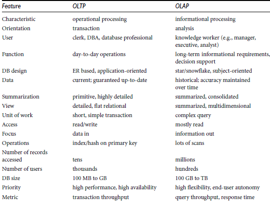
What is
the Difference Between OLAP and OLTP?
A data warehouse is a database containing data
that usually represents the business history of an organization. This
historical data is used for analysis that supports business decisions at many
levels, from strategic planning to performance evaluation of a discrete
organizational unit. Data in a data warehouse is organized to support analysis
rather than to process real-time transactions as in online transaction
processing systems (OLTP).
OLAP technology enables data warehouses to be
used effectively for online analysis, providing rapid responses to iterative
complex analytical queries. OLAP's multidimensional data model and data
aggregation techniques organize and summarize large amounts of data so it can
be evaluated quickly using online analysis and graphical tools. The answer to a
query into historical data often leads to subsequent queries as the analyst
searches for answers or explores possibilities. OLAP systems provide the speed
and flexibility to support the analyst in real time.
LECTURE-2
A MULTI-DIMENSIONAL DATA MODEL
n
A
data warehouse is based on a multidimensional data model which views data in
the form of a data cube as 3D,4D,nD .
n
A
data cube, such as sales, allows data to be modeled and viewed in multiple
dimensions
n
Dimension
tables are entities, such as item (item_name, brand, type), or time(day, week,
month, quarter, year)
n
Fact
table contains measures (such as dollars_sold)
n
Multidimensional data model is typically
organized around a central theme, like sales, for instance. This theme
is represented by a fact table. Facts are numerical measures.
n
Example:-sales
of a company
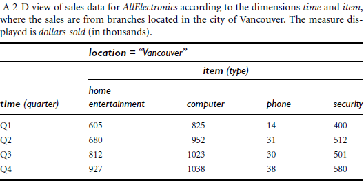
2 dimensions
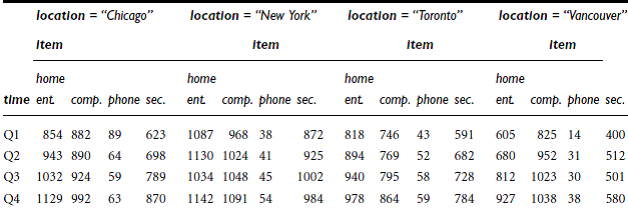
Ø 3-D
Example
of a 3-D view of sales data with dimension: Item, time, location
Fact
is sales (dollar_sold)
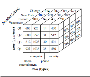
n
In
data warehousing literature, an n-D base cube is called a base cuboid. The top
most 0-D cuboid, which holds the highest-level of summarization, is called the
apex cuboid. The lattice of cuboids
forms a data cube.
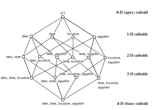
Ø
4-D and higher
dimensions.
Viewing things
in 4-d is difficult. We can think 4-d as series of 3-D cube.So for n-D data as
a series we can derive it as (n-1)-D cubes.
<<Derivation discussed in
Class>>
LECTURE-3
Schemas for
Multidimensional Databases
Multidimensional model can be
further divided into:- star schema, a snowflake schema, or a fact constellation
schema.
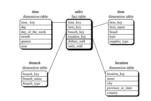
Star
schema:
The most common modeling paradigm is the star schema, in which the data
warehouse contains :-
(1) A large central table (fact
table) containing the bulk of the data, with no redundancy,
(2) A set of smaller dimension
tables, one for each dimension.
(3)1:1
The schema graph resembles a
starburst, with the dimension tables displayed in a radial pattern around the
central fact table.
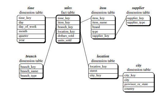
Snowflake
schema:
The snowflake schema is a variant of the star schema model
1.
Dimension
tables are normalized, thereby further splitting the data into
additional tables. The resulting schema graph forms a shape similar to a
snowflake.
2.
A
large central table (fact table)
3.
1:m(fact:dim)
Q)
Differentiate Between Star and Snowflake schema. Also suggest which is better
and why?
The major
difference between the snowflake and star schema models is that the dimension
tables of the snowflake model may be kept in normalized form to reduce redundancies.
Such a table is easy to maintain and saves storage space. However, this saving
of space is negligible in comparison to the typical magnitude of the fact table.
Furthermore, the snowflake structure can reduce the effectiveness of browsing, since
more joins will be needed to execute a query. Consequently, the system
performance
may be adversely
impacted. Hence, although the snowflake schema reduces redundancy, it is not as
popular as the star schema in data warehouse design.
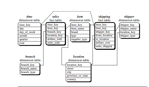
Fact
constellation(m:n)
Sophisticated applications may require multiple fact tables to share dimension
tables. This kind of schema can be viewed as a collection of stars, and hence
is called a galaxy schema or a fact constellation.
Application areas of these Schema’s:-where to use
which schema?
- A
data warehouse collects information about subjects that span the entire
organization, such as customers, items, sales, assets, and personnel,
and thus its scope is enterprise-wide. For data warehouses, the fact constellation schema is commonly
used, since it can model multiple, interrelated subjects.
- A
data mart, on the other hand, is a department subset of the data warehouse
that focuses on selected subjects, and thus its scope is departmentwide.
For data marts, the star or snowflake
schema are commonly used, since both are geared toward modeling single
subjects, although the star schema is more popular and efficient.
DMQL
(DATA MINING QUERY LANGUAGE)
Data warehouses and data marts
can be defined using two language primitives, one for cube definition and
one for dimension definition.
The cube
definition statement has the following syntax:
define cube <cube name>
[dimension list]: <measure list>
The
dimension definition statement has the following syntax:
define dimension <dimension
name>as <attribute or dimension list>
Eg:-
Ø Cube Definition
define cube sales star [time,
item, branch, location]:
dollars sold = sum(sales in
dollars), units sold = count(*)
Ø Dimension
Definition
define dimension time as (time
key, day, day of week, month, quarter, year)
define dimension item as (item
key, item name, brand, type, supplier type)
define dimension branch as
(branch key, branch name, branch type)
define dimension location as
(location key, street, city, province or state,country)
LECTURE_3
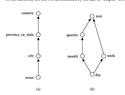
Concept
Hierarchies-A dimension can be further categorized from a set of
low level concept to high level concept.
This is called Concept Hierarchy.
Eg:-
Consider a
concept hierarchy for the dimension location.
City values for location
include Vancouver, Toronto, NewYork,and Chicago. Each city, however, can be
mapped to the province or state to which it belongs. These mappings form a concept hierarchy for
the dimension location, mapping a set of low-level concepts (i.e.,
cities) to higher-level, more general concepts (i.e., countries).
Typical OLAP Operations(refer to pg 124 for diagram)-v v
imp
1.
Roll up (drill-up): It is used to summarize data by climbing up hierarchy or by dimension
reduction .
When roll-up is performed by dimension reduction, one or more dimensions are
removed from the given cube
2.
Drill down (roll down): It is reverse of roll-up .We
move from higher level summary to
lower level summary or detailed data, or introducing new dimensions. Because a
drill-down adds more detail to the given data, it can also be performed by
adding new dimensions to a cube.
3.
Slice (select): The slice operation performs a selection on one dimension of the given
cube.
4.
dice: (project):
The
dice operation defines a sub
cube by performing a selection on two or more dimensions.
5. Pivot (rotate): reorient the
cube, change the dimensions and visualization, 3D to series of 2D planes
<Solved
all exercise examples related to OLAP OPERATIONS in class>
Lecture-4
Data
Warehouse Architecture
Business
Analysis Framework:
Four different
views regarding the design of a data warehouse must be considered for
Ø
The
top-down view allows the selection of the relevant information necessary for the
data warehouse. This information matches the current and future business needs.
Ø
The
data source view exposes the information being captured, stored, and managed by
operational systems. This information may be documented at various levels of
detail and accuracy, from individual
data source tables to integrated data source tables.
Ø
The
data warehouse view includes fact tables and dimension tables. It represents
the information that is stored inside the data warehouse, including pre
calculated totals and counts, as well as information regarding the source,
date, and time of origin, added to provide historical context.
Ø
Finally, the business query view is the
perspective of data in the data warehouse from
the viewpoint of the end user.
The Process of
Data Warehouse Design:
Ø There are two Approaches For Data warehouse Design- Top-down, bottom-up
approaches or a combination of both
n Top-down: Starts with overall design and planning and used where
technology is mature and well known.
n Bottom-up: Starts with experiments and prototypes .It is a rapid approach
and used for new and risky business applications.
Ø From software engineering point of view:
n Waterfall: structured and systematic analysis at each step before
proceeding to the next
n Spiral: rapid generation of increasingly functional systems, short turnaround
time, quick turnaround.
Steps For Data warehouse design process:
.png)
Because data warehouse construction is a difficult and long-term task, its implementation scope should be clearly defined. The goals of an initial data warehouse implementation should be specific, achievable, and measurable(SAM).
Lecture-5
Because data warehouse construction is a difficult and long-term task, its implementation scope should be clearly defined. The goals of an initial data warehouse implementation should be specific, achievable, and measurable(SAM).
Lecture-5
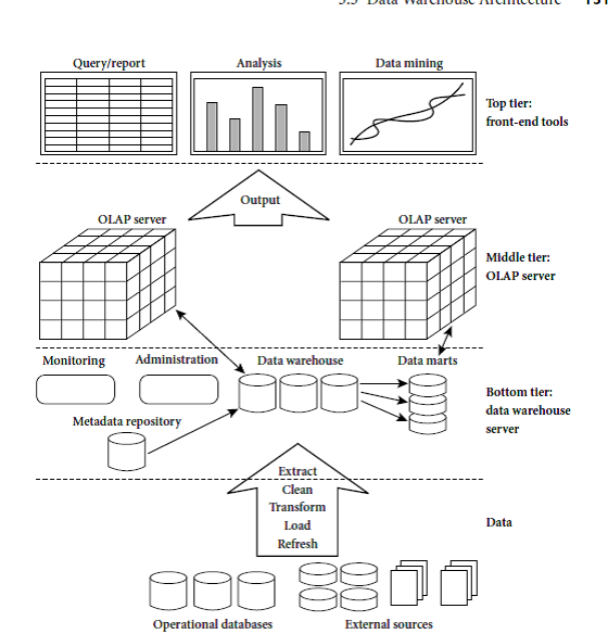
Data Warehouse: A Multi-Tiered Architecture
Ø BOTTOM TIER:
- It
is a warehouse database server. It contains Data Warehouse Back-End Tools
and Utilities.
- The
backend tools and utilities perform ETL (Extraction,Tranformation,Loading)process.
- Data
extraction-get data from multiple, heterogeneous, and external sources
- Data
cleaning-detect errors in the data and rectify them when possible
- Data
transformation-convert data from old format to warehouse format
- Load-Sort,
summarizes, consolidate, compute views, check integrity.
- Refresh-propagate
the updates from the data sources to the warehouse.
This bottom tier
also contains Metadata Repository
- Meta data is the data defining warehouse
objects. It stores: Description of
the structure of the data warehouse like schema, view, dimensions,
hierarchies, derived data definition, data mart locations and contents
- It
also contains Operational meta-data like old data (history of migrated data and
transformation path), currency of data (active, archived, or purged), monitoring
information (warehouse usage statistics, error reports, audit trails)
- The
algorithms used for summarization
- The
mapping from operational environment to the data warehouse
- Data
related to system performance, warehouse schema, view and derived data definitions
- Business
data-business terms and definitions, ownership of data, charging policies
Ø MIDDLE TIER-OLAP SERVERS
OLAP Servers Give Users Multidimensional
Data From Data warehouse Or data Marts.
Types of OLAP servers are:
n
Relational OLAP (ROLAP) –intermediate
servers
a)
Use
relational or extended-relational DBMS to store and manage warehouse data and
OLAP middle ware
b)
Include
optimization of DBMS backend, implementation of aggregation, navigation logic,
and additional tools and services
c)
Greater
scalability than MOLAP.
n
Multidimensional OLAP (MOLAP)
a)
They
support multidimensional views of data through array-based multidimensional
storage engine.
b)
They
map multidimensional views to data cube directly.
c)
They
are Fast indexing to pre-computed summarized data
n
Hybrid OLAP (HOLAP) (e.g.,
Microsoft SQLServer)
a)
Flexibility,
e.g., low level: relational, high-level: array
n
Specialized SQL servers (e.g.,
Redbricks)
a)
Specialized
support for SQL queries over star/snowflake schemas
Lecture-6
Three Data Warehouse Models: Architecture
point of views
- Enterprise
warehouse
a)
collects
all of the information about subjects spanning the entire organization
- Data Mart
a)
Subset of corporate-wide data that is of value
to a specific groups of users. Its scope
is confined to specific, selected groups, such as marketing data mart
b)
Independent
vs. dependent (directly from warehouse) data mart
- Virtual
warehouse
a)
A
set of views over operational databases
b)
Only
some of the possible summary views may be materialized
What is the Recommended Approach used
for development of a Data Warehouse?
“What are the pros and cons of
the top-down and bottom-up approaches to data warehouse development?”
The top-down development of an enterprise warehouse
serves as a systematic solution and minimizes integration problems.
However, it is expensive, takes a long time to develop, and lacks
flexibility due to the difficulty in achieving consistency and consensus for a
common data model for the entire organization.
The bottom-up approach to the design, development,
and deployment of independent data marts provides flexibility, low cost, and
rapid return of investment. It, however, can lead to problems when integrating
various disparate data marts into a consistent enterprise data warehouse.
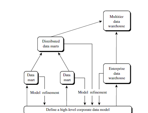
A recommended method for the development of data
warehouse systems is to implement the warehouse in an incremental and
evolutionary manner.
Steps:-
- First, a
high-level corporate data model is defined within a reasonably short
period (such as one or two months) that provides a corporate-wide, consistent,
integrated view of data among different subjects and potential usages
- Second,
independent data marts can be implemented in parallel with the enterprise
warehouse based on the same corporate data model set as above.
- Finally, a
multitier data warehouse is constructed where the enterprise warehouse is
the sole custodian of all warehouse data, which is then distributed to the
various dependent data marts.
Lecture-7
Ø Efficient Data Cube Computation
Data cube can be viewed as a
lattice of cuboids
- The bottom-most cuboid is
the base cuboid
- The top-most cuboid (apex)
contains only one cell
- How many cuboids in an
n-dimensional cube with L levels?
.png) |
4.
Cube
definition and computation in DMQL
define
cube sales[item, city, year]: sum(sales_in_dollars)
compute
cube sales
Transform
it into a SQL-like language (with a new operator cube by, introduced by Gray et
al.’96)
SELECT
item, city, year, SUM (amount)
FROM
SALES
CUBE BY item, city, and year
5.
Need
compute the following Group-Bys
(date,
product, customer),
(date,product),(date,
customer), (product, customer),
(date),
(product), (customer)()

Ø What
are the Various Data Warehouse Usage?
n
Three
kinds of data warehouse applications
1.
Information
processing
a)
supports
querying, basic statistical analysis, and reporting using crosstabs, tables,
charts and graphs
2.
Analytical
processing
a)
multidimensional
analysis of data warehouse data
b)
supports
basic OLAP operations, slice-dice, drilling, pivoting
3.
Data
mining
a)
knowledge
discovery from hidden patterns
b)
supports
associations, constructing analytical models, performing classification and
prediction, and presenting the mining results using visualization tools
From
On-Line Analytical Processing (OLAP) to On Line Analytical Mining (OLAM)
What is OLAM and Why online analytical mining is
important?
On-line analytical mining (OLAM) (also called OLAP
mining) integrates on-line analytical processing (OLAP) with data mining and
mining knowledge in multidimensional databases. Among the many different
paradigms and architectures of data mining systems, OLAM is particularly
important for the following reasons:
- High
quality of data in data warehouses: Most data mining tools need to work on
integrated, consistent, and cleaned data, which requires costly data
cleaning,data integration, and data transformation as preprocessing steps.
A data warehouse constructed by such preprocessing serves as a valuable
source of high quality data for OLAP as well as for data mining.
- Available
information processing infrastructure surrounding data warehouses: Comprehensive
information processing and data analysis infrastructures have been or will
be systematically constructed surrounding data warehouses
- OLAP-based
exploratory data analysis: Effective data mining needs exploratory data
analysis. A user will often want to traverse through a database, select
portion of relevant data, analyze them at different granularities, and
present knowledge/results in different forms.
Unit-2(last part)
Mining Frequent Patterns
What are
Frequent patterns and why are they important in data mining?
Frequent
patterns are
patterns (such as itemsets, subsequences, or substructures) that appear in a
data set frequently. For example, a set of items, such as milk and bread, that
appear frequently together in a transaction data set is a frequent itemset.
Ø
Finding
such frequent patterns plays an essential role in mining associations,
correlations, and many other interesting relationships among data. Moreover, it
helps in data classification, clustering, and other data mining tasks as well.
Ø
Frequent
itemset mining leads to the discovery of associations and correlations among items
in large transactional or relational data sets. With massive amounts of data continuously
being collected and stored, many industries are becoming interested in mining
such patterns from their databases. The discovery of interesting correlation relationships
among huge amounts of business transaction records can help in many business
decision-making processes, such as catalog design, cross-marketing, and
customer shopping behavior analysis.
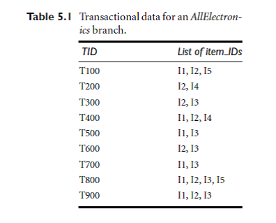
Market Basket
Analysis
A typical example of frequent item
set mining is market basket analysis. This process analyzes customer buying
habits by finding associations between the different items that customers place
in their “shopping baskets”
If we think of
the universe as the set of items available at the store, then each item has a
Boolean variable representing the presence or absence of that item. Each basket
can then be represented by a Boolean vector of values assigned to these
variables.
The Boolean
vectors can be analyzed for buying patterns that reflect items that are frequently
associated or purchased together. These patterns can be represented in
the form of association rules. For example, the information that customers who
purchase computers also tend to buy antivirus software at the same time is
represented in
Association
Rule below:
Computer->antivirus
software [support
= 2%; confidence = 60%]
Rule support and confidence are
two measures of rule interestingness
Ø Support 2% of
all the transactions under analysis show that computer and antivirus software
are purchased together.
Ø A confidence of
60% means that 60% of the customers who purchased a computer also bought the
software.
Ø support(A)B)
= P(AUB) )
Ø confidence(A)B)
= P(B/A)
ASSOCIATION
RULE MINING:-
Association rule mining can be
viewed as a two-step process:
1. Find all
frequent itemsets: By definition, each of these itemsets will occur at least
asfrequently as a predetermined minimum support count, min sup.
2. Generate strong
association rules from the frequent itemsets: By definition, these rules must
satisfy minimum support and minimum confidence.
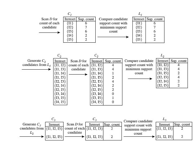
Efficient and
Scalable Frequent Itemset Mining Methods
Apriori is a algorithm proposed
by R. Agrawal and R. Srikant in 1994 for mining frequent itemsets for Boolean
association rules. The name of the algorithm is based on the fact that the
algorithm uses prior knowledge of frequent itemset properties.
The
Apriori Algorithm
Pseudo-code:
Ck: Candidate
itemset of size k
Lk : frequent
itemset of size k
L1 = {frequent
items};
for (k = 1; Lk
!=Æ;
k++) do begin
Ck+1 = candidates
generated from Lk;
for each transaction t in
database do
increment the count of all candidates in
Ck+1
that are contained in t
Lk+1 = candidates in Ck+1 with
min_support
end
return Èk Lk;
n
How
to generate candidates?
n
Step
1: self-joining Lk
n
Step
2: pruning
EXAMPLES:-GENERATE FREQUENT ITEM
SET AND ASSOCIATION RULES FROM THEM.
All numerical discussed in class.
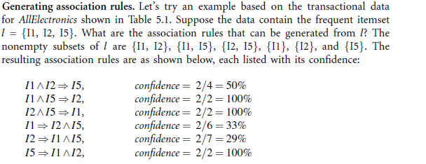
If the minimum
confidence threshold is, say, 70%, then only the second, third, and last rules
above are output, because these are the only ones generated that are strong.
Ways of Improving
the Efficiency of Apriori
“How can we
further improve the efficiency of Apriori-based mining?” Many variations
of the Apriori algorithm have been proposed that focus on improving the
efficiency of the original algorithm. Several of these variations are
summarized as follows:
- Hash-based
technique (hashing itemsets into corresponding buckets): A hash-based technique
can be used to reduce the size of the candidate k-itemsets, Ck,
for k > 1.
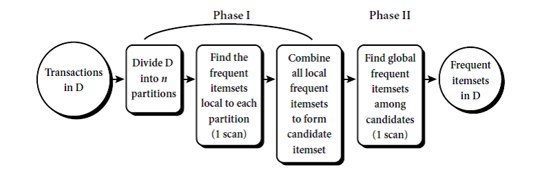
- Partitioning
(partitioning the data to find candidate itemsets): A partitioning
technique can be used that requires just two database scans to mine the
frequent itemsets. It consists of two phases. In Phase I, the algorithm
subdivides the transactions of D into n non overlapping
partitions. If the minimum support threshold for transactions in D is
min sup, then the minimum support count for a partition is min
sup_the number of transactions in that partition. For each
partition, all frequent itemsets within the partition are found. These are
referred to as local frequent itemsets. The procedure employs a special
data structure that, for each itemset, records the TIDs of the
transactions containing the items in the itemset. This allows it to find all
of the local frequent k-itemsets, for k = 1, 2, : : : , in
just one scan of the database.
- Sampling
(mining on a subset of the given data): The basic idea of the sampling approach
is to pick a random sample S of the given data D, and then
search for frequent itemsets in S instead of D.
FP-growth (finding frequent itemsets without
candidate generation).
n
Find
all frequent itemsets using FP Tree
TID
|
Items_bought
|
T1
T2
T3
T4
T5
|
M, O, N, K, E,
Y
D, O, N, K ,
E, Y
M, A, K, E
M, U, C, K ,Y
C, O, O, K, I
,E
|

K:5
E:4
M:3
O:3
Y:3
Rules:-
Y:
KEMO:1 KEO:1 KY:1
K:3 KY
O:
KEM:1 KE:2
KE:3 KO EO KEO
M:
KE:2 K:1
K:3 KM
E: K:4 KE
Why FP growth is
better than apriori algorithm?
- The
FP-growth method transforms the problem of finding long frequent patterns
to searching for shorter ones recursively and then concatenating the
suffix. It uses the least frequent items as a suffix, offering good
selectivity.
- The
method substantially reduces the search costs. cannot fit in main memory.
- A
study on the performance of the FP-growth method shows that it is
efficient and scalable for mining both long and short frequent patterns,
and is about an order of magnitude faster than the Apriori algorithm
From Association
Analysis to Correlation Analysis
There
are two methods of correlation analysis(Lift and Chi square)
- As
we have seen above, the support and confidence measures are insufficient
at filtering out uninteresting association rules. To tackle this weakness,
a correlation measure can be used to augment the support-confidence
framework for association rules. This leads to correlation rules of
the form
A->B [support,
confidence, correlation].
That is, a
correlation rule is measured not only by its support and confidence but also by
the correlation between itemsets A and B.
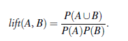
Lift is a simple
correlation measure that is given as follows. The occurrence of itemset A is
independent of the occurrence of itemset B if P(A UB)
= P(A)P(B); otherwise, itemsets A and B are
dependent and correlated as events. This definition can easily be extended to
more than two itemsets. The lift between the occurrence of A and B can
be measured by computing
If the resulting
value of lift is less than 1, then the occurrence of A is negatively correlated
with the occurrence of B. If the resulting value is greater than 1,
then A and B are positively correlated, meaning that the
occurrence of one implies the occurrence of the other. If the resulting
value is equal to 1, then A and B are independent and there
is no correlation between them.
Eg:-Calculate
the lift value for the following.
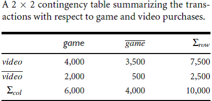
From the table, we can see that
the probability of purchasing a computer game is P(game) = 0:60,
theprobability of purchasing a video is P(video) = 0:75, and the
probability of purchasing both is P(game; video) = 0:40.),
The lift is P(game, video)/(P(game)xP(video))
= 0:40/(0:60X0:75) = 0.89. Because this value is less than 1, there is a
negative correlation between the occurrence of game and video.
- The
second correlation measure that we study is the chi square measure,
To compute the chisquare value,
we take the squared difference between the observed and expected value for a
slot (A and B pair) in the contingency table, divided by the expected value.
I had searched for many data warehouse consultant then I found your company to be the most effective service provider.
ReplyDeletebest
ReplyDeleteData warehouse architecture involves building the data warehouse in such a way that it collects and manages data efficiently. There are several layers involved in a data warehouse architecture. The highest layer is the interface. This refers to how the data warehouse communicates with the computer system. The second layer is the data environment. This refers to the database management system that stores the data warehouse. The lowest layer is the data. This refers to the raw data that is analyzed and stored in the database.
ReplyDeleteDWDM Unit 2 is an indispensable segment, delving into the intricacies of Dense Wavelength Division Multiplexing. Why Can't Support It demystifies complex concepts, providing a solid foundation.
ReplyDelete