.png)
+-+Copy.png)
UNIT-1
DATA MINING
What
Is Data Mining?
n
Data
mining (knowledge discovery from data) Extraction of interesting (non-trivial,
implicit, previously unknown and potentially useful)
patterns or knowledge from huge amount of data
n
Also
called as Knowledge discovery (mining) in databases (KDD), knowledge
extraction, data/pattern analysis, data archeology, data dredging, information
harvesting, business intelligence, etc
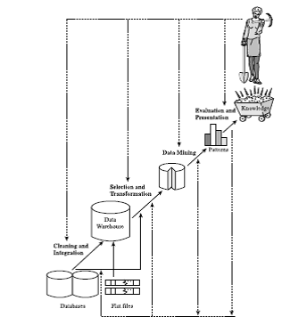
 Steps in Knowledge Discovery
1. Data cleaning (to remove noise
and inconsistent data)
2. Data integration (where multiple
data sources may be combined)
3. Data selection (where data
relevant to the analysis task are retrieved from the database)
4. Data transformation (where data
are transformed or consolidated into forms appropriate for mining by performing summary or aggregation operations,
for instance)
5.
Data mining (an
essential process where intelligent methods are applied in order to extract
data patterns)
6. Pattern evaluation (to identify
the truly interesting patterns representing knowledge based on some
interestingness measures;
7. Knowledge presentation (where
visualization and knowledge representation techniques are used to present the
mined knowledge to the user)
Q)Explain The architecture of a Typical Data mining
System
Architecture:
Typical Data Mining System
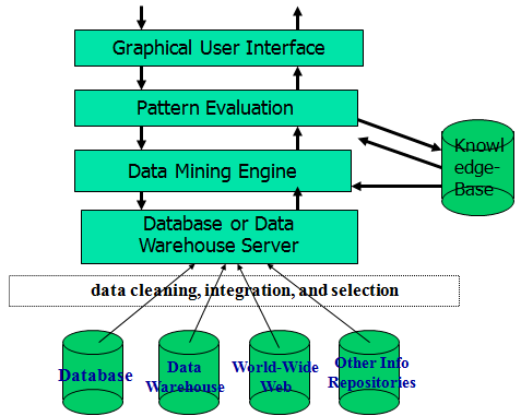
Components of a
data mining System
- Knowledge
base:
This is the domain knowledge that is used to guide the search or evaluate the interestingness of resulting
patterns. Such knowledge can include concept hierarchies, used to
organize attributes or attribute values into different levels of abstraction.
Knowledge such as user beliefs, which can be used to assess a pattern’s interestingness
based on its unexpectedness, may also be included
- Data mining
engine:
This is essential to the data mining system and ideally consists of a set
of functional modules for tasks
such as characterization, association and correlation analysis,
classification, prediction, cluster analysis, outlier analysis, and
evolution analysis.
- Pattern
evaluation module: This component typically employs
interestingness measures and interacts with the data mining modules so as
to focus the search toward interesting patterns. It may use interestingness
thresholds to filter out discovered patterns. For efficient data
mining, it is highly recommended to push the evaluation of pattern
interestingness as deep as possible into the mining process so as to
confine the search to only the interesting patterns.
- User
interface:
This module communicates between users and the data mining system, allowing
the user to interact with the system by specifying a data mining query or task,
providing information to help focus
the search, and investigating data mining based on the intermediate data
mining results. In addition, this component allows the user to browse
database and data warehouse schemas or data structures, evaluate mined
patterns, and visualize the patterns in different forms.
Lecture-2
On What Kind
Data Can we perform Data Mining?
Data Mining can
be performed on various types of data. These are Broadly divided into two
types. Database Oriented data sets and advanced Data sets.
n Database-oriented
data sets and applications
1. Relational database, data
warehouse, transactional database-RDBMS,DBMS
n Advanced
data sets and advanced applications
Ø Data streams and sensor data- huge or possibly infinite volume, dynamically changing, flowing in and
out in a fixed order, allowing only one or a small number of scans, and
demanding fast (often real-time) response time. Typical examples of data
streams include various kinds of scientific and engineering data, time-series data,
and data produced in other dynamic environments, such as power supply, network
traffic, stock exchange, telecommunications, Web click streams, video
surveillance, and weather or environment monitoring.
Ø
Temporal data- (incl. bio-sequences) A temporal
database typically stores relational data that include time-related attributes.
These attributes may involve several timestamps, each having different
semantics.
Ø
A
sequence database
stores sequences of ordered events, with or without a concrete notion of time.
Examples include customer shopping sequences, Web click streams, and biological
sequences.
Ø
A
time-series database
-stores sequences of values or events obtained over repeated measurements of
time (e.g., hourly, daily, weekly). Examples include data collected from the
stock exchange, inventory control, and the observation of natural phenomena
(like temperature and wind).
Ø
Object-relational
databases- This
model extends the relational model by providing a rich data type for handling
complex objects and object orientation.
Ø
Heterogeneous
databases and legacy databases
-A heterogeneous database consists of a set of interconnected, autonomous
component. A legacy database is a group of heterogeneous databases that
combines different kinds of data systems, such as relational or object-oriented
databases, hierarchical databases, network databases, spreadsheets, multimedia
databases, or file systems. The heterogeneous databases in a legacy database
may be connected by inter-computer networks
Ø
Spatial
data and spatiotemporal data
:Spatial databases contain spatial-related information. Examples include geographic
(map) databases, very large-scale integration (VLSI) or computer-aided design
databases, and medical and satellite image databases. A spatial database that
stores spatial objects that change with time is called a spatiotemporal
database, from which interesting information can be mined
Ø Multimedia database
Ø Text databases & WWW
Lecture-3
What are the
various Data Mining Functionalities/Task and What Kinds of Patterns Can Be
Mined?
Data mining tasks can be classified into two
categories: descriptive and predictive.
- Descriptive
mining tasks characterize the general properties of the data in the
database.
- Predictive
mining tasks perform inference on the current data in order to make
predictions.
- Concept/Class Description:
Characterization and Discrimination
Data can be
associated with classes or concepts.
For example, in the AllElectronics store, classes
of items for sale include computers and printers, and concepts of
customers include bigSpenders andbudgetSpenders. Concept of
students can be regular or irregular.
Such descriptions of a class or a concept are called
class/concept descriptions. These descriptions can be derived via
(1) data characterization, by summarizing the
data of the class under study and putting it in a target class.
(2) data discrimination, by comparison of the
target class with one or a set of comparative classes
(3) both data characterization and discrimination.
- Mining
Frequent Patterns, Associations, and Correlations
- Frequent
patterns, as the name suggests, are patterns that occur frequently in
data. There are many kinds of frequent patterns, including itemsets,
subsequences, and substructures.
- A frequent
itemset typically refers to a set of items that frequently appear
together in a transactional data set, such as milk and bread
Association analysis
:It is the analysis based on association Rules.
It can be single dimensional or multidimensional.
An example of such a rule, mined from the AllElectronics
transactional database, is
buys(X; “computer”))buys(X;
“software”) [support = 1%; confidence = 50%]where X is
a variable representing a customer. A confidence, or certainty, of 50% means that
if a customer buys a computer, there is a 50% chance that she will buy software
as well. A 1% support means that 1% of all of the transactions under analysis
showed that computer and software were purchased together.
Q) Explain this rule:-
A data mining system may find association rules like
age(X,
“20:::29”)^income(X, “20K:::29K”))buys(X, “CD
player”)[support = 2%, confidence = 60%]
Ans)The rule indicates that of the customers
under study, 2% are 20 to 29 years of age with an income of 20,000 to 29,000
and have purchased a CD player at AllElectronics. There is a 60%
probability that a customer in this age and income group will purchase a CD
player. Note that this is an association between more than one attribute, or
predicate (i.e., age, income, and buys). So it is
multidimensional.
- Classification
and Prediction
Classification is the process of
finding a model (or function) that describes and distinguishes data classes or
concepts, for the purpose of being able to use the model to predict the class
of objects The derived model is based on the analysis of a set of training data
(i.e., data objects whose class label is known).
Classification ModelsàIf then else,
decision Tree, Neural Networks.

- Cluster Analysis
The objects are clustered or
grouped based on the principle of maximizing the intraclass similarity and
minimizing the interclass
similarity. That
is, clusters of objects are formed so that objects within a cluster have high
similarity in comparison to one another, but are very dissimilar to objects in
other clusters. Each cluster that is formed can be viewed as a class of
objects. Examples: Group of customers in a city .
- Outlier Analysis
A database may contain data
objects that do not comply with the general behavior or model of the data.
These data objects are outliers. Most data mining methods discard outliers as
noise exceptions. However, in some applications such as fraud detection, the rare
events can be more interesting than the more regularly occurring ones. The
analysis of outlier data is referred to as outlier mining.
Lecture-4
Data
Mining Task Primitives
A data mining query is defined in
terms of data mining task primitives. These primitives allow the user to interactively
communicate with the data mining system.
Q)List and describe the five primitives for specifying
a data mining task.
The data mining
primitives are:-
- The
set of task-relevant data to be mined-This includes the database
attributes or data warehouse dimensions of interest (referred to as the relevant
attributes or dimensions)
- The
kind of knowledge to be mined: This specifies the data mining
functions to be performed, such as characterization, discrimination,
association or correlation analysis, classification, prediction,
clustering, outlier analysis, or evolution analysis.
- The background knowledge to be used in the discovery process.-use of concept hierarchy.
- The interestingness measures and thresholds for pattern evaluation-use of confidence and support.
- The
expected representation for visualizing the discovered patterns:
This refers to the form in which discovered patterns are to be displayed, which
may include rules, tables,charts, graphs, decision trees, and cubes.
Example:-
(1) use database
AllElectronics db ==================================> task
relevant
(2) use hierarchy location hierarchy for
T.branch, age hierarchy for C.age =======> background
knowledge.
(3) mine classification as promising
customers=======================> kind
of knowledge.
(4) in relevance to C.age,
C.income, I.type, I.placemade, T.branch
(5) from
customer C, item I, transaction T
(6) where I.item ID = T.item ID
and C.cust ID = T.cust ID and C.income _ 40,000 and I.price _ 100
(7) group by T.cust ID
(8) having sum(I.price) _ 1,000
Classification
of Data Mining Systems
- Classification
according to the kinds
of databases mined: A data mining system can be classified
according to the kinds of databases mined. Database systems can be
classified according to different criteria (such as data models, or the
types of data or applications involved), each of which may require its own
data mining technique. Data mining systems can therefore be classified
accordingly.
- Classification
according to the kinds
of knowledge mined: Data mining systems can be categorized
according to the kinds of knowledge they mine, that is, based on data
mining functionalities, such as characterization, discrimination,
association and correlation analysis, classification, prediction,
clustering, outlier analysis, and evolution analysis.
- Classification
according to the kinds
of techniques utilized: Data mining systems can be categorized
according to the underlying data mining techniques employed. These techniques
can be described according to the degree of user interaction involved.
- Classification
according to the applications
adapted: Data mining systems can also be categorized according
to the applications they adapt. For example, data mining systems may be
tailored specifically for finance, telecommunications, DNA, stock markets,
e-mail, and so on.
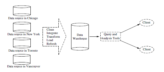
Integration
of a Data Mining System with a Database or DataWarehouse System
Q) How to integrate or couple the
DM system with a database (DB) system and/or a data warehouse (DW) system.
Ø
No coupling: No coupling means that a
DM system will not utilize any function of a DB or DW system.
Ø
Loose coupling: Loose coupling means
that a DM system will use some facilities of a DB or DW system, fetching data
from a data repository managed by these systems, performing data mining, and
then storing the mining results either in a file or in a designated place in a
database or data warehouse. Loose coupling is better than no coupling because
it can fetch any portion of data
stored
in databases or data warehouses by using query processing,
Ø
Semitight coupling: Semitight coupling means
that besides linking a DM system to a DB/DW system, efficient implementations
of a few essential data mining primitives.
Ø
Tight coupling: Tight coupling means
that a DM system is smoothly integrated into the DB/DW system. This approach is
highly desirable because it facilitates efficient implementations of data
mining functions, high system performance, and an integrated information processing
environment.
Another Probable Question
Describe the
differences between the following approaches for the integration of a data
mining system with a database or data warehouse system: no coupling, loose coupling, semitight
coupling, and tight coupling. State which approach you think is the
most popular, and why?
|
What are the Major Issues in Data
Mining?
Mining methodology and user interaction
issues:
Ø
Mining different kinds of knowledge in databases-Because
different users can be interested in different kinds of knowledge, data mining
should cover a wide spectrum of data analysis and knowledge discovery tasks.
These tasks may use the same database in different ways and require the
development of numerous data mining techniques.
Ø
Interactive mining of knowledge at multiple levels
of abstraction:
Because
it is difficult to know exactly what can be discovered within a database, the
data mining process should be interactive. Interactive mining allows users
to focus the search for patterns, providing and refining data mining requests
based on returned results.
Ø
Incorporation of background knowledge: Background
knowledge, or information regarding the domain under study, may be used to
guide the discovery process and allow discovered patterns to be expressed in
concise terms and at different levels of abstraction.
Ø
Handling noisy or incomplete data: The data stored
in a database may reflect noise, exceptional cases, or incomplete data objects.
When mining data regularities, these objects may confuse the process, causing
the knowledge model constructed to overfit the data.
Performance
issues: These include efficiency, scalability, and parallelization of data
mining algorithms.
Ø
Efficiency and scalability of data mining algorithms: To effectively
extract information from a huge amount of data in databases, data mining
algorithms must be efficient and scalable.
Ø
Parallel, distributed, and incremental mining
algorithms:
The
huge size of many databases, the wide distribution of data, and the
computational complexity of some data mining methods are factors motivating the
development of parallel and distributed data mining algorithms.
Issues
relating to the diversity of database types:
Ø Handling of
relational and complex types of data: Because relational databases and data
warehouses are widely used, the development of efficient and effective data
mining systems for such data is important.
Ø Mining
information from heterogeneous databases and global information systems: Local- and
wide-area computer networks (such as the Internet) connect many sources
of data, forming huge, distributed, and heterogeneous databases.
Data
Preprocessing
Ø What is dirty Data?
Data in the real world is dirty
which means that they are incomplete ,noisy and inconsistent.
1.
INCOMPLETE:
lacking attribute values, lacking certain attributes of interest, or containing
only aggregate data
a)
e.g., occupation=“ ”
b)
Incomplete data may come from “Not
applicable” data value when collected
c)
Human/hardware/software problems
2.
NOISY: containing errors or outliers e.g.,
Salary=“-10”
They arise due to Faulty data
collection instruments, Human or computer error at data entry Errors in data transmission
3.
INCONSISTENT:
containing discrepancies in codes or names
a)
e.g., Age=“42” Birthday=“03/07/1997”
b)
e.g., Was rating “1,2,3”, now rating “A,
B, C”
c)
e.g., discrepancy between duplicate
records
Ø
Why Is
Data Preprocessing Important?
No quality data leads to no
quality mining results. Quality decisions must be based on quality data.
e.g.,
duplicate or missing data may cause incorrect or even misleading statistics.
Data warehouse needs consistent integration
of quality data.
Ø What are the Major Tasks in Data
Preprocessing?
- Data
cleaning-Fill in missing values, smooth noisy data, identify or remove
outliers, and resolve inconsistencies
- Data
integration-Integration of multiple databases, data cubes, or files
- Data
transformation-Normalization and aggregation
- Data
reduction-Obtains reduced representation in volume but produces the same
or similar analytical results
- Data
discretization -Part of data reduction but with particular importance,
especially for numerical data
In summary, real-world data tend to be dirty,
incomplete, and inconsistent. Data preprocessing techniques can improve the
quality of the data, thereby helping to improve the accuracy and efficiency of the
subsequent mining process. Data preprocessing is an important step in the
knowledge discovery process, because quality decisions must be based on quality
data. Detecting data anomalies, rectifying them early, and reducing the data to
be analyzed can lead to huge payoffs for decision making.
Descriptive Data
Summarization
Defination:-Descriptive data
summarization techniques can be used to identify the typical properties of your
data and highlight which data values should be treated as noise or outliers.
It is of two types:-
- central
tendency include mean, median, mode, and midrange
- Dispersion
of the data. include quartiles, interquartile range (IQR), and variance.
Measuring the Central Tendency
.png) |
Mean:- .
Its of two types :-
n
Trimmed mean: chopping extreme values
and concentrating on the mean values only.
n
Mean is an algebraic measure.
Median:
Middle value if odd number of values or average of the middle two values
otherwise
Estimated by interpolation
- A holistic measure is a measure that must be computed on the entire data set as a whole. It cannot be computed by partitioning the given data into subsets and merging the values obtained for the measure in each subset. The median is an example of a holistic measure. Holistic measures are much more expensive to compute than distributive measures
.png)
Mode-Value that occurs
most frequently in the data
- Its
types are Unimodal, bimodal, trimodal
- Empirical formula: mean-mode=3*(mean-median)
Measuring
the Dispersion of Data
n
Quartiles, outliers and boxplots
1.
Quartiles: Q1 (25th
percentile), Q3 (75th percentile)
2.
Inter-quartile range: IQR = Q3 –
Q1
3.
Five number summary: min, Q1,
M, Q3, max
4.
Boxplot: ends of the box are the
quartiles, median is marked, whiskers, and plot outlier individually
5.
Outlier: usually, a value higher/lower
than 1.5 x IQR
n
Variance and standard deviation (sample:
s, population: σ)
1.
Variance: (algebraic, scalable computation)
.png)
n Standard deviation s (or σ) is the square root of variance s2 (or σ2)
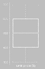
Box
plot Analysis
n
Five-number summary of a distribution:Minimum,
Q1, M, Q3, Maximum
n
Box plot
1.
Data is represented with a box
2.
The ends of the box are at the first and
third quartiles, i.e., the height of the box is IRQ
3.
The median is marked by a line within
the box
4.
Whiskers: two lines outside the box
extend to Minimum and Maximum
Numerical example:-
1. Suppose that the data for analysis includes the
attribute age. The age values for the data tuples are (in
increasing order) 13, 15, 16, 16, 19, 20, 20, 21, 22, 22, 25, 25, 25, 25, 30,
33, 33, 35, 35, 35, 35, 36, 40, 45, 46, 52, 70. (50 points)
(a) What is the mean of
the data? What is the median? What is the standard deviation?
Mean =
(13+15+16+16+19+20+20+21+22+22+25+25+25+25+
30+33+33+35+35+35+35+36+40+45+46+52+ 70) / 27 =
809/27 = 29.96
Median = middle value = 25
Standard deviation
Deviations from mean = {-16.96, -14.96, -13.96, -13.96,
-10.96, -9.96, -9.96, -8.96, -7.96, -7.96,-4.96, -4.96, -4.96,
-4.96, 0.04, 3.04, 3.04, 5.04, 5.04, 5.04, 5.04, 6.04, 10.04, 15.04, 16.04, 22.04,
40.04}
Squared deviations from mean = { 287.6416, 223.8016, 194.8816,
194.8816, 120.1216, 99.2016,
99.2016, 80.2816, 63.3616, 63.3616, 24.6016, 24.6016, 24.6016, 24.6016, 0.0016, 9.2416, 9.2416, 25.4016, 25.4016, 25.4016, 25.4016, 36.4816, 100.8016, 226.2016, 257.2816, 485.7616, 1603.2016}
Sum of squared deviations = 287.6416, 223.8016, 194.8816, 194.8816, 120.1216, 99.2016, 99.2016, 80.2816, 63.3616, 63.3616, 24.6016, 24.6016, 24.6016, 24.6016, 0.0016, 9.2416, 9.2416, 25.4016, 25.4016, 25.4016, 25.4016, 36.4816, 100.8016, 226.2016, 257.2816, 485.7616, 1603.2016= 4354.9632
Mean of squared deviations = 4354.9632/ 27 = 161.2949
Standard Deviation = √161.2949 = 12.7
What is the mode of the data? Comment on the
data's modality (i.e., bimodal, trimodal, etc.).
Mode = most frequent number = {25, 35}
Modality = bimodal
(b) What is the midrange of
the data?
Midrange = (13+70)/2 = 41.5
(c) Can you find (roughly) the 1st
quartile (Q1) and the third quartile (Q3) of the data?
Q1 =
median of lower half = 20 Q3 = median of upper half = 35
(d) Give the five-number
summary of the data.
min, Q1, median, Q3, max = 13, 20, 25, 35,
70
(e) If you plot a boxplot of
this data, what will be the box length (in actual number)? What min and max value would the whisker
extend to? Is there any outliner (i.e., elements beyond the extreme low and
high)?
Length = IQR = Q3-Q1 = 35-20 = 15
Min whisker = MAX(Q1 –
1.5 * IRQ, min) = MAX(20-1.5*15, 13) =
MAX(-2.5, 13) = 13
Max
whisker = MIN(Q3 + 1.5 * IRQ, max)
= MIN(35+1.5*15, 70) = MIN(67.5, 70) =
67.5
Outliers = anything higher than 67.5 or lower than 13 = {70}
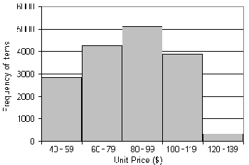
Graphic Displays of Basic Descriptive Data Summaries
Histogram: Plotting histograms, or frequency histograms, is a
graphical method for summarizing the distribution of a given attribute. A
histogram for an attribute A partitions the data distribution of A into
disjoint subsets, or buckets. Typically, the width of each bucket is
uniform. Each bucket is represented by a rectangle whose height is equal to the
count or relative frequency of the values at the bucket.
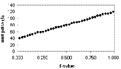
Quantile
plot: A quantile
plot is a simple and effective way to have a first look at a univariate data
distribution. First, it displays all of the data for the given attribute
(allowing the user to assess both the overall behavior and unusual
occurrences). Second, it plots quantile information.
Quantile-quantile
(q-q) plot: A quantile-quantile plot, or q-q plot, graphs the
quantiles of one univariate
distribution against the
corresponding quantiles of another. It is a powerful visualization tool in that
it allows the user to view whether there is a shift in going from one
distribution to another.
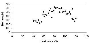
Scatter
plot: A scatter plot is one of the most effective graphical
methods for determining if there
appears to be a relationship,
pattern, or trend between two numerical attribute.
Loess
(local regression) curve: A loess curve is
another important exploratory graphic aid that adds a smooth curve to a scatter
plot in order to provide better perception of the pattern of dependence.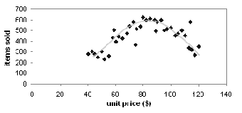
Ø What are the Major Tasks in Data
Preprocessing?
- Data
cleaning-Fill in missing values, smooth noisy data, identify or remove
outliers, and resolve inconsistencies
- Data
integration-Integration of multiple databases, data cubes, or files
- Data
transformation-Normalization and aggregation
- Data
reduction-Obtains reduced representation in volume but produces the same
or similar analytical results
- Data
discretization -Part of data reduction but with particular importance,
especially for numerical data
Data Cleaning
|
Data cleaning (or data cleansing) routines attempt to fill in
missing values, smooth out noise while identifying outliers, and correct
inconsistencies in the data.
Question: In real-world data, tuples with missing
values for some attributes are a common occurrence. Describe various
methods for handling this problem.
Answer: The various methods
for handling the problem of missing values in data tuples include:
(a) Ignoring the tuple: This
is usually done when the value is missing. This method is not very effective
unless the tuple contains several attributes with missing values. It is
especially poor when the percentage of missing values per attribute varies
considerably.
(b) Manually filling in the
missing value: In general, this approach is time-consuming and may not be a
reasonable task for large data sets with many missing values, especially when
the value to be filled
in is not easily determined.
(c) Using a global constant to
fill in the missing value: Replace all missing attribute values by the same
constant, such as a label like \Unknown," Hence, although this
method is simple, it is not recommended.
(d) Using the attribute mean
for quantitative (numeric) values or attribute mode for categorical (nominal)
values: For example, suppose that the average income of AllElectronics customers
is $28,000. Use this value to replace any missing values for income.
(e) Using the most probable
value to fill in the missing value
Q:How do we remove Noisy Data?
Noise is random error or
variance in a measured variable. It is a disturbance. The various reasons for
noise are:
n Incorrect attribute values may due to
1.
faulty data
collection instruments
2.
data entry
problems
3.
data transmission
problems
4.
technology
limitation
5.
inconsistency in
naming convention
n Other data problems which requires data cleaning
1.
duplicate records
2.
incomplete data
3.
inconsistent data
The various methods of data smoothing and removing noise
are:-
- Binning
a) first sort data and partition
into (equal-frequency/equal -width) bins
b) then one can smooth by bin
means, smooth by bin median, smooth by
bin boundaries, etc.
Q: Suppose a group of 12 sales price
records has been sorted as follows:
5; 10;
11; 13; 15; 35; 50; 55; 72; 92;
204; 215:
Partition
them into three bins by each of the following methods.
(a)
equal-frequency partitioning
(b)
equal-width partitioning
Answer:
(a)
equal-frequency partitioning
bin 1
5,10,11,13
bin 2
15,35,50,55
bin 3
72,92,204,215
(b)
equal-width partitioning
The
width of each interval is (215 - 5)/=3 = 70.
bin 1
5,10,11,13,15,35,50,55,72
bin 2
92
bin 3
204,215
- Regression : Data can be smoothed by fitting the data to a
function, such as with regression. Linear regression involves
finding the “best” line to fit two attributes (or variables), so that one
attribute can be used to predict the other.
- Clustering-detect and remove
outliers-Outliers may be detected by clustering, where
similar values are organized into
groups, or “clusters.” Intuitively, values that fall outside of the set of
clusters may be considered
Q:Explain Data Cleaning as a Process
The first step in data
cleaning as a process is discrepancy detection. Discrepancies can be
caused by several factors, including poorly designed data entry forms that have
many optional fields, human error in data entry, deliberate errors (e.g.,
respondents not wanting to divulge information about themselves), and data
decay (e.g., outdated addresses).Discrepancies may also arise from inconsistent
data representations and the inconsistent use of codes.
Discrepancy can be solved by
the following methods:-
- Use
metadata (e.g., domain, range, dependency, distribution)
- Check
field overloading
- Check
uniqueness rule, consecutive rule and null rule
- Use
commercial tools:-
a)
Data scrubbing:
use simple domain knowledge (e.g., postal code, spell-check) to detect errors
and make corrections
b)
Data auditing: by
analyzing data to discover rules and relationship to detect violators (e.g.,
correlation and clustering to find outliers)
DATA INTEGRATION
|
Data
integration, combines data from multiple sources into a coherent
data store, as in data warehousing. These sources may include multiple
databases, data cubes, or flat files.
Q:Discuss issues to consider during data integration.
Answer: Data integration
involves combining data from multiple sources into a coherent data store.
Issues that mustbe considered during such integration include:
- Entity-Identification problems/ Schema integration: The metadata from the different data
sources must be integrated in order to match up equivalent real-world
entities.
- Handling
redundant data: Derived attributes may be redundant, and inconsistent
attribute naming may also lead to redundancies in the resulting data set.
Duplications at the tuple level may occur and thus need to be detected and
resolved.
- Detection
and resolution of data value conficts: Differences in representation,
scaling, or encoding may cause the same real-world entity attribute values
to differ in the data sources being integrated.
Redundancy is another important issue:
Some redundancies can be
detected by correlation analysis. Given two attributes, such analysis can
measure how strongly one attribute implies the other, based on the available data.
For numerical attributes, we can evaluate the correlation between two
attributes, A and B, by computing the correlation coefficient.
n Correlation coefficient (also called Pearson’s product
moment coefficient)
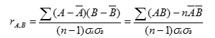
where n is
the number of tuples, respective means of A and B, σA and σB are the respective
standard deviation of A and B, and Σ(AB) is the sum of the AB cross-product.
- If rA,B > 0, A and B are positively
correlated (A’s values increase as B’s).
The higher, the stronger correlation.
- rA,B = 0: independent; rA,B < 0: negatively correlated
n Χ2 (chi-square) test
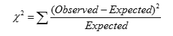 |
n The larger the Χ2 value, the more
likely the variables are related
DATA TRANSFORMATION
|
In data transformation,
the data are transformed or consolidated into forms appropriate for mining.
Data transformation can involve the following:
- Smoothing,
which works to remove noise from the data. Such techniques include binning,
regression, and clustering.
- Aggregation,
where summary or aggregation operations are applied to the data. For example,
the daily sales data may be aggregated so as to compute monthly and annual
total amounts. This step is typically used in constructing a data cube for
analysis of the data at multiple granularities.
- Generalization
of the data, where low-level or “primitive” (raw) data are replaced by higher-level
concepts through the use of concept hierarchies. For example, categorical attributes,
like street, can be generalized to higher-level concepts, like city
or country. Similarly, values for numerical attributes, like age,
may be mapped to higher-level concepts, like youth, middle-aged,
and senior.
- Normalization,
where the attribute data are scaled so as to fall within a small specified
range, such as 1:0 to 1:0, or 0:0 to 1:0.
- Attribute
construction (or feature construction),where new attributes are
constructed and added from the given set of attributes to help the mining
process.
Data
Transformation: Normalization techniques
- Min-max
normalization: to [new_minA, new_maxA]
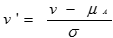
·
Z-score normalization (μ: mean, σ: standard deviation):
·
Normalization by decimal scaling

DATA
REDUCTION STRATEGIES
|
Data reduction techniques can be applied to obtain a
reduced representation of the data set that is much smaller in volume, yet
closely maintains the integrity of the original data.
Strategies for data reduction include the following:
1. Data cube aggregation, where
aggregation operations are applied to the data in the construction of a data
cube.
2. Attribute subset selection, where irrelevant, weakly relevant, or redundant
attributes or dimensions may be detected and removed. The following are the
methods:-
i). Stepwise forward selection: The procedure starts with an empty set of attributes
as the reduced set. The best of the original attributes is determined and added
to the reduced set. At each subsequent iteration or step, the best of the
remaining original attributes is added to the set.
ii). Stepwise backward elimination: The procedure starts with the full set of attributes.
At each step, it removes the worst attribute remaining in the set.
iii). Combination of forward selection and backward
elimination: The stepwise forward selection and backward
elimination methods can be combined so that, at each step, the procedure
selects the best attribute and removes the worst from among the remaining
attributes.
3. Dimensionality reduction, where encoding mechanisms are used to reduce the data set
size. In dimensionality reduction, data encoding or
transformations are applied so as to obtain a reduced or “compressed”
representation of the original data. If the original data can be reconstructed
from the compressed data without any loss of information, the data reduction
is called lossless. If, instead, we can reconstruct only an approximation of the
original data, then the data reduction is called lossy. Two popular and
effective methods of lossy dimensionality reduction: wavelet transforms and
principal components analysis
4. Numerosity reduction, where the
data are replaced or estimated by alternative, smaller data representations
such as parametric models (which need store only the model parameters instead
of the actual data) or nonparametric methods such as clustering, sampling, and
the use of histograms.
Sampling
Sampling can be used as a data reduction technique
because it allows a large data set to be represented by a much smaller random
sample (or subset) of the data. Suppose that a large data set, D,
contains N tuples
Simple random sample without replacement (SRSWOR) of
size s: This is created by drawing s
of the N tuples from D (s < N), where the
probability of drawing any tuple in D is 1=N, that is, all tuples
are equally likely to be sampled.
Simple random sample with replacement (SRSWR) of size s: This is similar to SRSWOR, except that each time a tuple
is drawn from D, it is recorded and then replaced. That is, after
a tuple is drawn, it is placed back in D so that it may be drawn again
5. Discretization and concept hierarchy generation,where raw data values for attributes are replaced by
ranges or higher conceptual levels Discretization and concept hierarchy
generation are powerful tools for data mining, in that they allow the mining of
data at multiple levels of abstraction. Discretization techniques can be
categorized based on how the discretization is performed, such as whether it
uses class information or which direction it proceeds (i.e., top-down vs.
bottom-up)
life saver
ReplyDelete